Operations with Columns

The Reports tool enables the user to execute the following operations with columns:

There are two ways to insert a column:

Insert to the Left. A new column is added to the left of the current one. The new column width is the same as the width of the column to the left of the current one.
Insert to the Right. A new column is added to the right of the current one. The new column width is the same as the width of the current one.

To add a new column, select an existing column, or any cell in the column, and execute one of the following operations:

Select the Insert Column Left or Insert Column Right item in the column header context menu.
Select the Insert > Insert Column Left or Insert > Insert Column Right context menu item of the cell contained in the column.
Select the Insert > Insert Column Left or Insert > Insert Column Right item in the Cells group on the Home ribbon tab.
Press ALT+T. A column is added to the left of the selected cell or column.

NOTE. If before adding a column filtering was set up for the range, it is also applied for a new column.

The columns to the right of the new column are shifted one position to the right. When a column is inserted to the left, all the columns, starting from the selected one, are shifted. When a column is inserted to the right, the selected column stays in its place, and the columns to the right of it are shifted.

Multiple columns can be added at the same time. In this case, the number of inserted columns matches the number of initially selected columns.

There are three ways to change column width:

Changing Width Manually. To manually change column width, point to the right column border in the header area and drag the border to the required position while holding down the mouse button. When the mouse pointer appears as a two-headed arrow, you can click and drag an item:

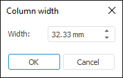
Exact Width Change. To specify exact column width, select required column (or any cell in this column) and select the Format > Column Width item in the Cells group of the Home ribbon tab. A dialog box with the same name opens after executing the command:

In the dialog box that opens enter (or edit) the value to set for all columns that cross the currently selected range. The same operation can be executed by using the Column Width context menu item of column(s) name.

NOTE. The value can be entered in different measurement units. The editor box shows values using measurement units that correspond to the current regional settings of the operating system.

Automatic. In addition to manual change, you can automatically fit the column width to the optimum size for the cell contents. To do this, select a column or a group of columns, and then select the Format > Autofit Column Width item in the Cells group of the Home ribbon tab. The column width is set to the minimum required to display the longest text line in the column. The condition is also satisfied when a single cell is selected. This method of changing column width has the following features:
- Width autofit ignores the cells with the text wrap configured, as these cells fit to virtually any column width.
- When width of merged cells is adjusted automatically, first the width is calculated for unmerged cells in the range, and then for merged cells.

Another quick way to adjust column width automatically is double-clicking the two-headed arrow. The mouse cursor changes to such an arrow when it is hovered over the border between column headers.

Each of these methods can be applied to a single column or a column group.

Column hiding can be used when columns contain intermediate results. The data stored in hidden columns is not shown in the screen or on a printed sheet.

To hide a column, select required column or any cell in this column, and execute one of the following operations:

Select the Hide context menu item of column header.
Select the Format > Hide or Show > Hide Columns item in the Cells group of the Home ribbon tab.

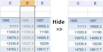
After executing one of these commands the selected column is hidden. The column at its right takes place of the hidden column:

Multiple columns can be hidden at the same time.

To show a hidden column, select two columns: column at the left and at the right of the hidden one, and then:

Select the Show context menu item of selected columns' headers.
Select the Format > Hide or Show > Show Columns item in the Cells group of the Home ribbon tab.

After this, the hidden columns between the selected columns are shown:

If several hidden columns are positioned between the selected columns, the Show command shows all the hidden columns.

If it is required to display all hidden columns on the sheet, before executing the command select the whole sheet.

NOTE. Setting zero width for a column and hiding it are different operations.

To delete a column, select an existing column, or any cell in the column, and execute one of the following operations:

Select the Delete > Delete Columns item in the column context menu.
Select the Delete > Delete Columns context menu item of the cell contained in the column.
Select the Delete > Delete Columns item in the Cells group of the Home ribbon tab.

The column is deleted even if only a single cell has been selected in this column. After executing this command the selected column is deleted, and all the columns to the right of it shift one position to the left.

Multiple columns can be deleted at the same time. To do this, before executing the operation select the range including at least one cell of each of the deleted columns.

Variables in formulas are replaced in the following way:

When a column is deleted, all values that contain name of this column in their name, are replaced with "#REF!" in the formula. The cell values, which formulas contain references to the deleted column, are replaced with "#REF!".
All values that have in their names a letter, which is closer to the beginning of alphabet than the deleted column letter, remain unchanged.
All values that contain a letter that is closer to the end of the alphabet, than the deleted column letter, are shifted one letter closer to the A (F1 is replaced with E1, E1 is replaced with D1, and so on).

When you delete columns in the sheet, check if data areas are included in the range to delete. A confirmation is required if the range to be deleted contains one or more data area. After confirming the operation, the data areas are deleted both from the sheet and the report. The data areas deleted in this way, are not shown in the Data Sources and Data Slices panel.