Formatting Cells Based on Their Values

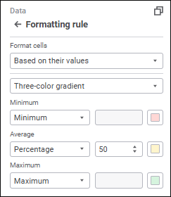
It formats cell values using three colors: minimum value color, average value color, and maximum value color. Intermediate colors are calculated automatically depending on cell values.

Set three assessment points: Minimum, Average, and Maximum. These points determine the range of values to be formatted. Therefore, formatting will be applied to the table cells, which values are included in the specified range.

Specify for each point:

• Value. Point value. Value format depends on its type.

• Color. Point color.

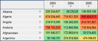
The example of conditional formatting, in which cells with minimum value are green, cells with average value are yellow, and cells with maximum value are red. Colors for values that are greater or less than the average are calculated automatically:

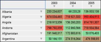
It formats cell values using two colors: minimum value color and maximum value color. Intermediate colors are calculated automatically depending on cell values.

Set two assessment points: Minimum and Maximum. These points determine the range of values to be formatted. Therefore, formatting will be applied to the table cells, which values are included in the specified range.

Specify for each point:

• Value. Point value. Value format depends on its type.

• Color. Point color.

The example of conditional formatting, in which cells with minimum value are green and cells with maximum value are red. Intermediate value colors are calculated automatically:

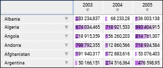
It displays histograms in cells that correspond to the value: the greater is the value, the bigger is the chart. For example:

Set two assessment points: Minimum and Maximum. These points determine the range of values to be formatted. Therefore, formatting will be applied to the table cells, which values are included in the specified range.

Specify for each point:

• Value. Point value. Value format depends on its type.

Determine general formatting style settings:

• Color. Histogram color.

• Show Value. The checkbox is selected by default, and cells show histograms and their values. If the checkbox is deselected, cells show only histograms.

They divide cell values into several groups. The icon indicates whether the cell is included in a group.

Set the following parameters:

• Set. Select the used icons set.

• Icon Application Rules. Set assessment points. The number of points matches the number of icons in the selected set. The rules are applied from top to bottom.

Specify for each point:

1. • Condition. Set the condition to define the values corresponding to the point.

   • Value. Point value. Value format depends on its type.

   • Type. Value type:

   • Number. Point value is set as a specific number.

   • Percentage. Point value is set as a percentage of the maximum value contained in the formatted table. The range of available values: [0, 100].

   • Formula. Point value is set as a formula. Numbers, round brackets, and arithmetic operations signs can be used in a formula. If an invalid formula is entered in the Value box, the box will be highlighted. For details see the Formula Creation Rules section.

   • Percentile. Point value is set as a percentile. For example, the percentile equal to 75 is the value, below which there are 75% of values of the formatted table.

NOTE. The application rule for the last assessment point is created automatically.

• Reverse Order of Icons. The checkbox is deselected by default, and icons are applied in the specified order. When the checkbox is selected, icons will be applied in the reverse order.

• Show Values. The checkbox is selected by default, and cells show icons and values. If the checkbox is deselected, cells show only icons.

The example of formatting, in which cells are divided into three groups: average values, values greater than average, and values less than average.