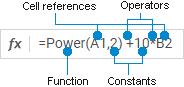
Formulas are expressions, by which data is transformed into another type.
Any formula starts with an equality sign (=):
The following is used in the formula:
Built-in function.
Cell references: A1 and B2 return the values contained in corresponding cells.
Constants: numeric or text values entered to the formula, for example, 2 and 20.
Operators: + – addition sign and * – multiplication sign.
It can be used in formula:
A constant is a ready (not calculated) value. Examples of constants: date 10.10.2015, number 210 and text "Quarterly profit". Expression or its value are not constants.
If a formula does not contain references to other cells (for example, a formula looks as =30+70+110), value in such cell is changed only after manual changing of the formula.
Operators are operations that must be executed with formula operands. There is a standard order of calculation execution but it can be changed by means of brackets.
When creating formulas in regular reports one can use various types of operators: arithmetic operators, comparison operators.
They are used to execute arithmetic operations: addition, subtraction, multiplication. Operations are executed with numbers. The following arithmetic operators are available:
| Operation sign | Description |
| + | Addition. |
| - | Subtraction. |
| * | Multiplication. |
| / | Division. |
They are used to compare two values. Comparison results in the logical value: True or False.
| Operation sign | Description |
| = | Equal. |
| < | Less. |
| > | Greater. |
| <= | Less than or equal. |
| >= | Greater than or equal. |
| <> | Greater than or less than (not equal). |
Special features of using references to cells of report sheet in a formula:
Single Cell. Specify address of a sheet cell, such as B8.
Column. To use all cells of a column in a formula, specify its name via a colon, for example: B:B. To use all cells of several columns, specify their name via a colon, for example: A:C.
Row. To use all cells of the same row, specify its number via a colon, for example: 5:5. To use all cells of several rows, specify their name via a colon, for example: 1:5.
Cell Range. To use a cell range in a formula, first specify address of the upper left cell, where the range starts, next, after a colon, specify address of the bottom right cell where the range ends, for example:
C7:D15
Where:
C7. The address of the upper left cell.
D15. The address of the lower right cell.
Combined cell range. To describe the area that contains several non-intersecting ranges (including single cells), specify addresses of rectangular areas and single cells via a semicolon. For example:
C7:D15;A1:B4;B8
Where:
C7:D15 and A1:B4. Cell ranges.
B8. Single cell.
Referring to the cells of another sheet. To use a cell or a cell range located on another sheet, specify sheet name in quotation marks and with an exclamation mark before the range.
A link to a sheet is inserted following these steps:
The sheet name is inserted into cursor position when the user moves to another sheet. If a term was selected, sheet name is inserted into selected term position. No objects are selected on the active sheet.
Select the required cell or cell range on the sheet - references to a cell or cell range are inserted into cursor position. The cell or cell range is marked with a dashed frame.
Changing the active sheet adjusts sheet name in the resulting term, the reference to range is not adjusted, it corresponds to selection on each of the activated sheets. Changing borders of the range selected on the active sheet results in adjusting the reference to this range in the resulting term.
When the active sheet changes, the cursor remains within the cell editor or in the formula bar, depending on its position before this event.
If the formula is entered using the cell editor, and another sheet is activated or a term is inserted on entering the formula, when the user goes back to the current sheet, the editor is restored, and the cursor is put after the added term.
After the formula is entered, the sheet, to which the formula was entered, becomes active.
Formula editing stops when another sheet is activated if:
The cursor is put after any term.
The cursor is within a term.
Several characters that are not a term are selected: a cell address (A0) and a sheet name with the exclamation mark (“Sheet1”!).
If other sheets are activated when the formula is being entered, the current sheet is highlighted. References to other sheets in the formula or on the sheet are not highlighted in color. Examples of references:
="Sheet1"!A3
Value of the A3 cell from the sheet 1.
=Sum("Sheet2"!A:A)
Sum of value of the A column from the sheet 2.
=Sum("Sheet3"!C31;A31;E31)
Sum of the combined range: the value of the C31 cell is taken from the sheet 3, while values of the A31 and E31 cells are taken from the current sheet.
=Sum("Sheet2"!B31:D31)
Sum of value range from the sheet 2.
To specify cell or range references, use the mouse or type the address using the keyboard, provided that the first character in the cell should be the equality sign. To specify the combined range of cells using the mouse, hold down the CTRL key.
The selected cell or cell range is highlighted using a dashed color frame. When entering operators or signs separating function parameters, the cell is fixed and highlighted using a solid color frame. The next mouse click specifies the address of another cell. Use the mouse to move, increase or decrease a highlighted cell or cell range, the formula address automatically changes. To increase or decrease the range, hover the cursor over the cell corner and after it changes to a two-headed arrow drag the range border in the required direction.
The entered or edited cell or cell range address and the appropriate cell or cell range borders have the same color.
NOTE. If it is required to use circular references in formulas, select the Iterative Calculations checkbox on the Formulas tab on the Parameters panel. By default, such formulas are not calculated, and the cells display the following error message: "Circular references are found". Examples of circular references: the =C11+ B9 + A0 formula is defined for the A0 cell; and the following formulas are defined for three cells: A0 (=A1 + 1), A1 (=A2 + 1), A2 (=A0 + 1).
Two reference styles can be used when creating references in regular reports:
A1. When the A1 style is used, columns are marked with letters and rows are marked with numbers.
R1C1. When the R1C1 style is used, rows and columns are marked with numbers, and references for cells in formulas are set by shifting from the current cell. For example, the R[-1]C[2] cell refers to the cell one row to the top and two columns to the right of the current cell.
When reference style changes, references are automatically converted into the selected style.
One can use only one reference style in reports.
The reference style to be used for visual composition of formulas is determined in regular report settings.

 Absolute and relative references
The following reference types can be used to create formulas:
Relative reference in a formula, for example, A1, is based on the position of the cell that contains the formula, and the cell, to which the formula refers. When position of the cell containing the formula changes, the reference changes too. When the formula is copied or filled along rows and columns, the reference is automatically corrected.
Absolute reference of a cell in a formula, for example, $A$1, always refers to the cell located on a certain sheet. When position of the cell containing the formula changes, the absolute reference does not change. When the formula is copied or filled along rows and columns, the absolute reference is not corrected. It is available for the A1 style.
Mixed reference contains either an absolute column and a relative row, or an absolute row and a relative column. When position of the cell containing the formula changes, the relative reference is changed and the absolute reference does not change. When the formula is copied or filled along rows and columns, the relative reference is automatically corrected and the absolute reference is not corrected.
Depending on reference style the way of indicating absolute and relative references differs:
A1 style. If the A1 style is used for specifying absolute references, use the $ sign. To fix reference in the cell or formula bar:
Enter the $ character before the reference part that should be fixed.
Press F4: single-clicking fixes the cell, double-clicking fixes the row, triple-clicking fixes the column, four times clicking makes the reference relative again. The cell next to the cursor is fixed, select the entire formula to fix all references in the cell.
=$A1
When this reference is copied, the A column is always fixed. Relative part of the reference, that is, row number changes according to the row, to which the reference is copied (=$A2, =$A3, and so on).
R1C1 style. When the R1C1 style is used, to specify absolute references one should specify number of the row or column after the R or C letters. Relative numbers of rows and columns are enclosed in square brackets and correspond to the shift relative to the current cell. To fix reference in the cell or formula bar:
Enter numbers of rows/columns in square brackets.
Press F4: single-clicking fixes the cell, double-clicking fixes the row, triple-clicking fixes the column, four times clicking makes the reference relative again. The cell next to the cursor is fixed, select the entire formula to fix all references in the cell.
When this reference is copied, the relative number does not change, but in fact it corresponds to another row or column.
=R[-3]C0
When copied, this reference has the same appearance, but on calculation the reference corresponds to the cell positioned in the first column three rows above the formula cell.
The =$A$0 absolute reference created with the use of the A1 style is identical to the =R0C0 reference created with the use of the R1C1 style.
The =RC1 reference created with the use of the R1C1 style is identical to reference to the cell located in the RC column and in the first row created with the use of the A1 style.
Functions are predefined formulas that execute calculations by specified values named arguments in the determined order. Functions can be used to execute simple and complex calculations.
To add a built-in function to the formula, open the function wizard. The following function categories are available:
Some functions return the array of values (for example, MInverse, MMult), so they should be entered as array formulas. To insert an array formula:
Enter functions to a cell by using function wizard or keyboard.
Select the cell range (array), which will store the calculation result, starting from the cell containing the formula.
Press F2, then press CTRL+SHIFT+ENTER.
After executing the operations, the area displays the value array returned by the function.
If, while defining the cell range (Step 2), the area greater than the returned array was selected, the extra cells will display the #N/A value. If the area less than the returned array was selected, only part of the array will be displayed.
NOTE. To delete the array formula, select the cell range with the formula. On an attempt to edit or delete the formula, an error message is displayed in the part of the array.
Fore functions connected to report
Connect the development environment object containing the implementation of the required function. Public access modifier must be used for the formula.
To use the Fore function in a formula, specify the expression in the cell after the = character: <Unit identifier>.<Function name>[(<Function parameter values>)].
For example, custom function in the unit with the MODULE identifier looks as follows:
Public Function My(Value: Integer): Integer;
Begin
Value := Value + 50;
Return Value;
End Function My;
To use the custom function, enter the expression into the selected cell:
=MODULE.My(50)
After the calculation the selected cell shows the 100 value.
Custom functions can be used to enhance regular report capabilities due to the use of custom calculation methods.
Examples of formulas:
=12*B2+C3/2
=Abs(A0)
=Sum(K10:K15)+20
=B0+"Sheet2"!A1
NOTE. When exporting to *.xls note that not all functions are supported in Microsoft Excel.
The following operations are available when working with formulas:
A formula can be created in the following ways:
Directly in the cell. To do this, execute the following operations in the cell to edit:
Enter the equality sign. Skip this step if the cell already contains this sign.
Create a formula using numbers, statements, cell references and functions. When a function is entered, its autocompletion is available.
Press the ENTER key to save and calculate the formula.
In the formula bar.
By using the function wizard. To do this, click the  Insert Function button in the formula bar or press SHIFT+F3.
By copying the cell with the created formula. Execute the following operations:
To cancel entering formula, press the ESC key.
A formula can be edited:
Directly in the cell. To do this, in the edited cell:
Edit the formula using numbers, statements, cell references and functions. When a function is entered, its autocompletion is available.
Press the ENTER key to save and calculate the formula.
In the formula bar.
By using the function wizard. To do this, click the Insert Function button in the formula bar or press SHIFT+F3.
To cancel entering formula, press the ESC key.
View formula intermediate value
To view formula intermediate value:
Select the cell with the formula.
In the formula bar select the part, for which one should view intermediate result.
Press F9. Intermediate result is displayed instead of the selected formula part.
Save:
Formula's intermediate result. Press the ENTER key, and intermediate result will replace the selected formula part.
Formula. Press the ESC key, and the selected formula part will be restored.
To use hints during entering formulas, open the Formulas tab on the Settings panel and select the Formula Autocompletion checkbox.
If the property is set to True, the cell or formula bar displays the functions, which names contain the entered sequence of characters. A short description is displayed for each function.
To navigate along the list, use the UP and DOWN keys. To select the function, use the TAB key or double-click the function.
To set up indication of the cells with errors, go to the Formulas tab on the Settings tab and select the Error Checking checkbox.
NOTE. If multiple error cells with errors are selected, the error identifier is shown for the upper left range cell. The Ignore Error and Error Checking Options commands are available for several cells.
See also:
Working with Report Sheet | Formula Bar | Function Wizard