Interpolation (Web Application)

Interpolation

The method calculates data of a lower level based on upper level data. It is used in problems that require data disaggregation. For example, when it is required to distribute quarterly frequency data by months.

NOTE. To disaggregate data, calendar frequency of the input variable must be greater than that of the output variable. If calendar frequency of the input variable is smaller or the same as output variable frequency, the user cannot create the Interpolation equation.

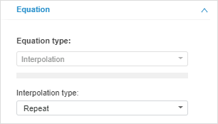
To set up method parameters, use the Equation side panel tab.

Make sure that the side panel is displayed.
Select the output variable or one of the connections of equation of the Interpolation type.
Go to the Equation side panel tab.

Interpolation Type. Specify interpolation type that is applied to the input variable. If the method has parameters, the box to enter their values is displayed. Available interpolation types:

Repeat. Values of output frequency repeat the existing values of the original variable frequency. The method has no parameters.

Uniform. Modeling is executed using uniform interpolation. Each original frequency point is uniformly split into output frequency points. For example, quarterly data for 2008 is calculated by splitting up annual data for 2008 into four equal parts. The method has no parameters.

Linear. Output frequency values are calculated using an equation of a line, which connects existing points of original frequency. The method has no parameters.

Geometric. Output frequency values are in proportion to the increment value and are in inverse proportion to the factor calculated based on the increment. Increment is exponentially dependent on the logarithm of the original frequency relative to the increment multiplied by the length of the output frequency period. The method has no parameters.

Cubic Splines. Output frequency values are calculated using the equation of a curve, which passes through a set of points in such a way that the first curve derivatives and the second curve derivatives are continuous at each point. This curve is created by a series of cubical polynomials passing through sets of three adjacent points. Then cubical polynomials are joined together to create a single curve. The method has no parameters.

Lagrange Polynomial. This method is used to determine a multinomial, which value is 1 at one node point and 0 at the rest of the points. The method has no parameters.

Polynomial. Modeling is executed using the specified degree polynomial interpolation. Polynomial degree is set in the Polynomial Degree value editor. Minimum value of the polynomial degree is one.

Pattern. Modeling is executed using pattern interpolation. Set the Pattern Type and the Pattern Series parameters. Use the Pattern Type drop-down list to specify the pattern to be used for interpolation. Available patterns:

Average by Elements.
By First Element.
By Last Element.

Select the variable representing a pattern data series in the Pattern Series hierarchical list.

To set the pattern series:

- Select the variable in the data view area (the Schema view).
- Hold down the mouse button and drag the variable to the Pattern Series box.
- Release the mouse button. Values of the variable are used to substitute the missing data.

To remove the pattern series, click the button.

First. Value of the first output frequency point matches the point value at the original frequency. Other values of the output frequency points remain empty.

Last. Value of the last output frequency point matches the point value at the original frequency. Other values of the output frequency points remain empty.