This type of formatting condition is used to format cells satisfying the specified formula.
For example, the cells with values that satisfy the formula Value>B1 are formatted in the table:

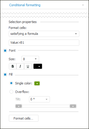
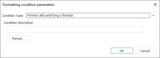
To set up formatting of the cells satisfying the specified formula, use the Conditional Formatting tab on the side panel or the Formatting Condition Parameters dialog box.


NOTE. Setting up using the side panel is available only in the Analytical Queries (OLAP) tool.
Set formula, based on which cells to be formatted are calculated.
Determine formatting settings:
Font. Select the checkbox to determine font settings in the cells with formatted values. Set font size, style and color in cells in appropriate boxes.
Fill. Select the checkbox to determine fill settings in the cells with formatted values. Set fill type:
Single Color. Solid cell fill. Select fill color in the drop-down palette.
Overflow. Two-color gradient is used to fill cell background. Select the start and end colors of the gradient in the appropriate drop-down palettes. Use the Tilt box to set gradient tilt angle.
Format Cells. Click the button to set up additional formatting parameters for cells with definite values. The Formatting dialog box opens.
NOTE. The option is available only in the desktop application.
To create a formula, follow the rules:
A formula can contain constants, operators, built-in functions.
The Value keyword can be used in a formula. When calculating a formula the current cell value is placed instead of this word.
One can use in formula cell references, A1 and R1C1 reference styles, absolute and relative references, development environment functions.
NOTE. It is available only in the Reports tool.
Examples of formulas:
Value>1000
Abs(Value)
Sum(K10:K15)+20
If the formula is formed incorrectly, it is highlighted:

See also: