Singular spectrum analysis (SSA) belongs to distribution-free methods of time series analysis. The method is aimed at decomposing a time series into interpretive additive components. The method does not require stationarity of a series, trend model awareness, and information about periodic components in the series. Having such weak statements the method can solve various problems, for example, trend discrimination, finding periodic component, series smoothing.
Because of absence of the model the possibility to check a hypothesis about existence of some component in a series, but based on the information, obtaining using the analysis, a parametric model to check hypothesis can be built.
Basic algorithm of the method consists of two complementary steps: decomposition and recovery.
Assume that F = (f1, …, fn) is a real length time series N (N > 2 ). The F series is non-zero, that is, there is at least one i that the fi ≠ 0.
Nesting
At this step, the input time series is transformed to a sequence of multidimensional vectors.
Assume that L is the length of such vectors: integer number, determined by a user (1 < L < N). Nesting procedure forms K = N - L + 1 vectors of nesting
![]()
Therefore, L is received - trajectory matrix of series F: X = [X1; …; XK], which consists of nesting vectors as columns.
Singular Decomposition
Assume that S = (1/K)XXT. Suppose that λ1; …; λL - proper names of the S matrix taken in descending order (λ1 ≥ … ≥ 0); U = [U1; …; UL] - orthogonal system of proper vectors of the S matrix corresponding to proper names.
The U matrix can be considered as the matrix of transition to main components XU = Y = (y1, …, yL).
Main Components Recovery
Because of properties of the U matrix it is possible to present matrix of the X series as X = YU'. Therefore, we get decomposed matrices of a series by main components. Decomposition can be obtained, using not all main components, but only those, which contain the biggest part of information about series. In this case columns of Y matrix, corresponding to minor components, are filled with zeroes.
Recovery of One-Dimensional Series
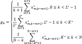
Recovery is executed using procedure of diagonal averaging.
Assume that L* = min(L, K), K* = max(L, K), where L x K is dimensions of matrix X. Then suppose that x*ij = xij, if L < K, and x*ij = xji when otherwise. The procedure of diagonal averaging transfer matrix X to an output series G = (g0, …, gN-1) by the following formulas:

Therefore, basic algorithm enables the user to smooth F input series, rejecting its random value (noise).
See also: