 Insert rows
The Reports tool enables the user to execute the following operations with rows:
There are two ways to insert a row:
Insert Row Below. The new row is added under the current one. Height of the added row will match the current row height.
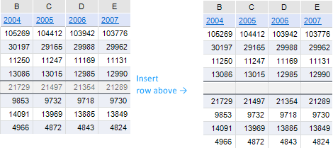
Insert Row Above. The new row is added above the current one. Height of the added row will match height of the row above the current one.
To add a new row, select an existing row, or any cell in the row, and execute one of the following operations:
Select the Insert Row Above and Insert Row Below item in the row header context menu.
Select the Insert > Insert Row Above or Insert > Insert Row Below context menu item of the cell contained in the row.
Select the Insert > Insert Row Above or Insert > Insert Row Below item in the Cells group on the Home ribbon tab.
Press ALT+Y. A row above the selected cell or row is added.
NOTE. If before adding a row filtering was set up for the table, it is also applied to a new row.
After executing this command, a new row is added into specified position, and the existing row moves to the opposite direction:

Multiple rows can be added at the same time. The number of inserted rows matches the number of initially selected rows.
There are several ways to change row height:
Changing Height Manually. To manually change row height, hover the cursor on the bottom border of the row in the header area. The cursor changes to a two-headed arrow (indicating that movement is possible), click the mouse button and drag the border to the required distance while holding down the mouse:

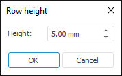
Exact Height Change. To specify exact row height, select required row (or any cell in this row) and execute the Format > Row Height item in the Cells group of the Home ribbon tab. A dialog box with the same name opens after executing the command:

In the dialog box enter (or edit) the value to set for the current row or selected rows. The same operation can be executed by selecting the Row Height context menu item of row(s) name.
NOTE. The value can be entered in different measurement units. The editor box shows values using measurement units that correspond to the current regional settings of the operating system.
Row Autoheight. You can also autofit row height to fit cell contents. To do this, select a row or a group of rows, and then execute the Format > Autofit Row Height item in the Cells group of the Home ribbon tab. After executing this command the row height is set to fit the highest line in the text. This method of changing row height has the following features:
When the height is selected automatically, the cells with the text wrap configured are ignored, as these cells can fit to virtually any row height.
When the height of a merged cell is adjusted automatically, the height is calculated for unmerged cells first and for the merged cell after that.
Quick Row Height Fit. To quickly fir row height, put the cursor to the row border until the cursor changes to a two-headed arrow. Double-click the row border in row headers area.
NOTE. When changing row height consider the following features of text wrap in cells:
• If row cell height was not changed manually, selecting the radio button Word Wrap or Use Hyphenation automatically autofits cell height.
• Chinese text is wrapped by hieroglyphs.
Each of these methods can be applied to one row or a row group.
Row hiding can be used when rows contain intermediate results. The data stored in hidden rows is not shown in the screen or on a printed sheet.
To hide a row, select required row or any cell in this row, and execute one of the following operations:
Select the Hide item in the row heading context menu.
Select the Format > Hide or Show > Hide Rows item in the Cells group of the Home ribbon tab.
After executing this command the selected row is hidden. The row below it takes its place.
Multiple rows can be hidden at once.
To show a hidden row, select the rows above and below the hidden one, and then:
Select the Show context menu item of selected rows' headers.
Select the Format > Hide or Show > Show Rows item in the Cells group of the Home ribbon tab.
The hidden row between the selected rows is shown.
If several hidden rows are positioned between the selected rows, the Show command shows all the hidden rows.
To display all the hidden rows on the sheet, select all the rows of the sheet and select the Display context menu item of the row headers area.
To delete a row, select required row (or any cell in this row), and execute one of the following operations:
Select the Delete > Delete Rows item in the row header context menu.
Select the Delete > Delete Rows context menu item of the cell contained in the row.
Select the Delete > Delete Rows item in the Cells group of the Home ribbon tab.
The row is deleted even if only one row cell is selected. After executing this command the selected row is deleted. The row below it takes its place.
Multiple rows can be deleted at once. To do this, before executing the operation, select a range that contains at least one cell of each of the rows to delete.
Variables in formulas are replaced in the following way:
When a row is deleted, all values that contain number of this row in their name, are replaced with "#REF!" in the formula. The cell values, which formulas contain references to the deleted row, are replaced with #REF!.
All values containing in their names a number that is less than the number of deleted row, remain unchanged.
All the values that have the number greater than the number of the deleted row in their name are reduced by one (A10 is replaced with A9, B10 with B9, and so on).
When rows are deleted, the system corrects formulas that include deleted (moved as a result of adding) cells located on other sheets of the regular report.
On deleting rows in the sheet, check if data areas are included in the range to delete. A confirmation is required if the range to be deleted contains one or more data area. After confirming the operation, the data areas are deleted both from the sheet and the report. The data areas deleted in this way are not shown in the Data Sources and Data Slices panel.
The first row in the sheet can be frozen to always show the fixed area in the screen on data scrolling.
To freeze the first row, select the Freeze Areas item in the Window group of the View ribbon tab, and select the Freeze First Row menu item.
To unfreeze areas, select the Freeze Areas item in the Window group of the View ribbon tab, and select the Unfreeze Areas menu item.
See also:
Getting Started with the Reports Tool in the Web Application | Working with Reports Sheet Elements