
 To display the tab
To set up output model data transformation, use the Transformations side panel tab.
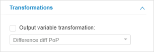
If the output variable data needs to be transformed, select the corresponding checkbox and select one of the methods.
The following transformations can be applied to variables:
None. No transformation (default value).
Natural Logarithm log. The logarithm of output variable points is found: ln(X[t]).
Logarithms Difference. A difference of logarithms is found for neighboring points of the output variable for a certain period (ln(X[t]/X[t-N])):
dlog PoP. Previous period.
dlog YoY. Corresponding period of the previous year.
dlog YTD. End of the previous year.
Rate of Change. The rate of change is calculated to the previous period (in percents) (X[t]/X[t-N]-1)*100):
pch PoP. Previous period.
pch YoY. Corresponding period of the previous year.
pch YTD. End of the previous year.
Difference. The transformation y[t] = X[t] – X[t-N] is executed for a given period:
diff PoP. Previous period.
diff YoY. Corresponding period of the previous year.
diff YTD. End of the previous year.
Normalization norm. Points of the output variable are normalized: X[t]/σ(X) where σ is root-mean-square deviation of the series.
Standardization std. Points of the output variable are standardized: (X[t]-M(X))/σ(X), where σ is root-mean-square deviation of the series, M - average of the series.
Growth Coefficient. The growth rate is calculated for a certain period (X[t]/X[t-N]):
ratio PoP. Previous period.
ratio YoY. Corresponding period of the previous year.
ratio YTD. End of the previous year.
Annual Rate of Change (pchA). Annual rate of change is calculated in percents: (((X[t]/X[t-1])^S)-1)*100, where S is the number of periods in a year.
Trend Subtract. Trend is subtracted using the formula: X[t]-f(X(t), S), where f(X(t), S) series trend, S - trend type:
(Linear Trend) TS Linear.
(Polynomial Trend) TS Polynomial.
(Logarithmic Trend) TS Logarithmic.
(Inverse Trend) TS Inverse.
Seasonal Adjustment. Seasonality is adjusted using the Census1 method based on the formula that depends on seasonality type:
(Auto) SA Auto. Iff(X>=0,SA Multiplicative, SA Additive), X - all series values. If the series does not include negative values, seasonality type is multiplicative; if it does, seasonality type is additive.
(Additive) SA Additive. Additive seasonality: SA(X[t])=X[t]-s1(X[t]), where s1 is the seasonal component of the series X[t].
(Multiplicative) SA Multiplicative. Multiplicative seasonality: SA(X[t])=X[t]/s2(X[t])*100, where s2 is the seasonal component of the series X[t].
The seasonal period is determined on equation frequency (quarter or month).
Outlier Adjustment OA. Outliers are adjusted using the k-sigma method: X[t]-f(X(t), K), where f(X(t), K) is outlier of the series X(t), K is calculation parameter by k-sigma method.
See also: