Formatting Cells Based on Their Values

This type of formatting condition is used to format all selected cells by their values.

To set up formatting of the cells by their values, use the Conditional Formatting tab on the side panel or the Formatting Condition Parameters dialog box.

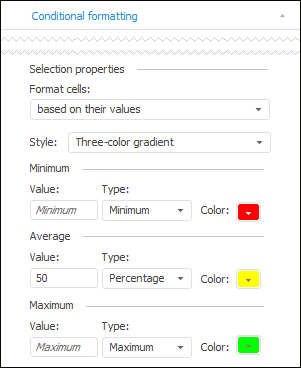
The set of options depends on the selected formatting style. To select the style, use the Style drop-down list.

Available styles:

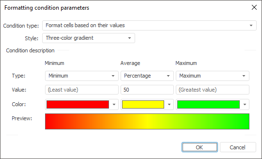
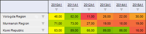
Three-Color Gradient

It formats values in cells based on three colors: color corresponding to minimum value; color corresponding to average value, and color corresponding to maximum value. Intermediate colors are calculated automatically based on cell values.

The example of conditional formatting, in which cells with minimum values are red, with average values are yellow, and with maximum values are green. Colors for the values above or below the average are calculated automatically:

Style settings:

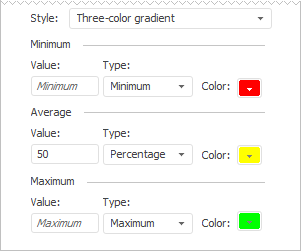
Set three estimate points: Minimum, Average and Maximum. These points will set the range of values to format. Thus, formatting is applied for the table cells, which values are located in the specified range.

Specify for each point:

• Value. A value that corresponds to the point. Value format depends on its type.

• Color. A color that corresponds to the point.

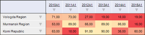
Two-Color Gradient

It formats values in cells based on two colors: color corresponding to minimum value and color corresponding to maximum value. Intermediate colors are calculated automatically based on cell values.

The example of conditional formatting, in which cells with minimum values are red and with maximum values are yellow. Colors for intermediate values are calculated automatically:

Style settings:

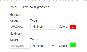
Set two estimate points: Minimum and Maximum. These points will set the range of values to format. Thus, formatting is applied for the table cells, which values are located in the specified range.

Specify for each point:

• Value. A value that corresponds to the point. Value format depends on its type.

• Color. A color that corresponds to the point.

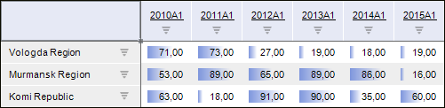
Histograms

It displays histograms in cells that correspond to the value: the greater is the value, the larger is the histogram. For example:

Style settings:

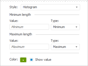
Set two estimate points: Minimum and Maximum. These points will set the range of values to format. Thus, formatting is applied for the table cells, which values are located in the specified range.

Specify for each point:

• Value. A value that corresponds to the point. Value format depends on its type.

Determine general formatting style settings:

• Color. Histogram color.

• Show Value. The checkbox is selected by default, and histograms and values are shown in cells. If the checkbox is deselected, only histograms are shown in cells.

Icons

It divides cell values into several groups. The cell that belongs to a certain group is indicated with the appropriate icon.

The example of formatting, in which cells are divided into three groups: average values, values above average, values below average:

Style settings:

Set the following parameters:

• Scope. Select the scope of icons to use.

• Icons Application Rules. Set estimate points. The number of points matches the number of icons in the selected scope. Specify for each point:

• • Rule. Set the rule to identify values that correspond to the point.

  • Value. A value that corresponds to the point. Value format depends on its type.

  • Type. Value type:

  • Minimum. It is available only for the Minimum point. This type automatically determines the minimum value contained in the formatted table. Manual entering of values is not available.

  • Number. The point value is set as a particular number.

  • Percentage. The point value is set as percentage from the maximum value contained in the formatted table. Range of available values: [0; 100].

  • Formula. The point value is set as a formula. A formula can contain numbers, round brackets and arithmetic operators. If an incorrect formula is entered in the Value box, it is highlighted.

  The example of the Formula value type use.

• NOTE. See formula creation rules in the Formula Creation Rules section.

• Percentile. The point value is set as a percentile. For example, the percentile that is equal to 75 is the value, below which 75% of values are taken in the formatted table.

• Maximum. It is available only for the Maximum point. This type automatically determines the maximum value contained in the formatted table. Manual entering of values is not available.

1. The Minimum and Maximum types are not available for the Icons style.

NOTE. The application rule for the last estimate point is automatically formed.

• Reverse Order of Icons. The checkbox is deselected by default, and icons are applied in the specified order. If the checkbox is selected, icons are applied in the reverse order.

• Show Values. The checkbox is selected by default, and icons and values are shown in cells. If the checkbox is deselected, only icons are shown in cells.

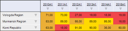
Fill by Groups

The style divides cell values into several groups. The cell that belongs to a certain group is indicated with the appropriate color.

The example of formatting, in which cells are divided into three groups: average values are yellow, values above average are orange, values below average are red:

Style settings:

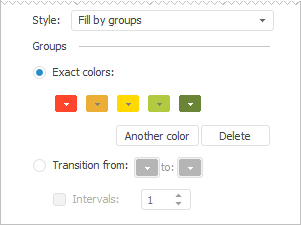
Set color selection mode for groups of values:

• Exact Colors. Each group color is set manually by means of the drop-down palette.
  To add a new group, click the Another Color button. A new palette is added. Select the required color in it.
  To delete the last group, click the Delete button. The group is deleted without confirming the deletion request.

• Transition from. Group colors are set by means of two-color gradient. Select the start and the end colors of the gradient in the drop-down palettes. To set the number of groups, select the Intervals checkbox and specify the required number of groups. If the checkbox is deselected, the number of groups is automatically determined.

Example of the Formula Value Type Use

In the example for regular report, the conditional formatting as three-color gradient using the Formula value type is created:

NOTE. See formula creation rules in the Formula Creation Rules section.