Interpolation

Interpolation is a method of finding secondary value data points within the range of a discrete set of known data points.

Interpolation uses function values specified for a number of points to predict the function values between them. The methods listed below are used to create a series with higher observation frequency based on a series with lower frequency. For example, to calculate a series with quarterly frequency based on annual data.

Suppose there is a system of distinct points xi(i ϵ 0, 1, …, N) that belong to some range G. The values of the f function are known only for the following points: yi = f(xi), i = 1, …, N.

Interpolation process finds such a function f in the specified class of functions, that F(xi) = yi,  i = 1, …, N.

The points xi are interpolation nodes, while a collection of these points is an interpolation grid.

The pairs (xi, yi) are data points or basic points.

The difference between neighbor values ∆xi = xi -xi - 1   is interpolation grid step. The step can be changeable or constant.

The function F(x) is named an interpolating function (interpolant).

Linear Interpolation

Linear interpolation links existing data points M(xi, yi) (i = 0, 1, ..., n) with straight lines, and the function f(x) approximates toward a broken line with nodes at these points.

Generally, equations of each segment of a broken line are different. As there are n intervals (xi, xi+1), for each of these intervals an equation of a straight line is used that crosses two points, as the interpolation polynomial equation. Particularly, for the i-th interval the user can write an equation of a straight line that crosses the points (xi, yi) and (xi+1, yi+1), as:

Therefore:

Geometric Interpolation

If geometric interpolation is used, values of output frequency are proportionate to the increment value and are inversely proportional to the factor calculated based on the increment. The increment is exponentially dependent on the logarithm relative to the source frequency increment multiplied by the length of the output frequency period.

Consider geometrical method on the example of calculating quarterly data based on annual data.

• X[t] – source annual data.

• Inc[t] = exp(log(X[t+1] / X[t]) / 4) – increment value.

• Factor[t] = (1 + Inc[t] + Inc[t]^2 + Inc[t]^3) / 4 – factor value.

• X[t,1], X[t,2], X[t,3], X[t,4] – quarterly data in the year t.

Therefore:

• X[t,1] = X[t] / Factor[t].

• X[t,2] = X[t] * Inc[t] / Factor[t].

• X[t,3] = (X[t] * Inc[t]^2) / Factor[t].

• X[t,4] = (X[t] * Inc[t]^3) / Factor[t].

Interpolation for other frequencies is made in the similar way.

Cubic Spline Interpolation

Splines are used to effectively handle observed experimental dependencies between parameters that have a rather complex structure. Due to their ease of use, cubic splines are most frequently used. Basic concepts of cubic spline theory were developed as a result of attempts to mathematically describe flexible splines made from elastic material (mechanical splines) that have been used by designers to draw a sufficiently smooth curve crossing the certain points. An elastic spline, which is fixed at some points and is in equilibrium, takes the shape, which enables it to minimize its energy. Due to this fundamental property, splines can be effectively used to solve real-world problems of processing experimental information.

Usually, it is required to find the y = ϕ(x) approximation for the function y = f(x), so that f(xi) = ϕ(xi) at the points x = xi, and at other points of the [a, b] segment values of the functions f(x) and ϕ(x) are close. If experimental points are few (for example, 6-8), the user can use one of the interpolation polynomial methods to solve an interpolation problem. However, if there are a lot of calculated points, interpolation polynomials become close to useless. This is due to the fact that the degree of an interpolation polynomial is less than the number of experimental function values only by one. Though, of course, the function segment can be split into portions including a small number of experimental points, and interpolation polynomials can be calculated for each of these segments. But in this case the approximation function has points where the derivative is not continuous, that is, function graph has salient points.

Cubic splines are free from this drawback. Researches of the beam theory have shown that a flexible thin beam between two nodes is rather well described by a cubic polynomial, and since it is not destroyed, the approximating function should be at least continuously differentiable. This means that the functions ϕ(x), ϕ'(x), ϕ''(x) should be continuous at the interval [a, b].

The cubic interpolation spline that corresponds to the given function f(x) and the given nodes xi, is the function S(x), that satisfies the following conditions:

• At each segment of [xi-1, xi], i = 1, 2, ..., n the function S(x) is a third degree polynomial.

• The function S(x), as well as its first and second derivatives are continuous at the interval [a, b].

• S(xi) = f(x), i = 0, 1, ..., n.

At each of the segments [xi-1, xi], i = 0, 1, ..., n we find the function S(x) = Si(x) as a third degree polynomial:

The condition of continuity for all derivatives up to the second degree is written as:

Interpolation condition:

ai, bi, ci, di - spline coefficients that need to be defined at all n linear elements:

Edge conditions of the spline c0 and cn:

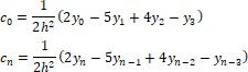
If the function f(x) is a third (or smaller) degree polynomial, the data is reproduced more accurately if the border conditions of the spline c0 and cn are equal to precise values of the second derivative of the cubic polynomial.

Lagrange Polynomial Interpolation

The Lagrange polynomial is the minimum degree polynomial that takes given values at the given set of points. For n + 1 pairs of values (x0, y0), (x1, y1), …, (xn, yn), where all xi are different (i = 0, 1, ..., n), there is only one polynomial L(x) with the degree not greater than n, for which L(xi) = yi.

In the simplest case (n = 1) it is a linear polynomial, and its graph is a straight line that crosses two selected points.

Lagrange proposed a method for calculating these polynomials:

Where basis polynomials are calculated as:

lj(x) have the following properties:

• n degree polynomials.

• lj(xj)= 1.

• lj(xi) = 0 when i ≠ j.

This means that L(x), as a linear combination of lj(x), cannot have a degree greater than n, and L(xj) = yj.

Polynomial Interpolation

Polynomial interpolation is the best known method of one-dimensional interpolation. The method advantages are the ease of use and good quality of resultant interpolants.

This method describes a n-th degree polynomial P0, 1, …, n-1, n, that crosses n points (from 0-th ton-th), as a function of two n-1 degree polynomials following the formula:

The same formula is recursively applied to the obtained polynomials, until the user gets polynomials of the type Pi calculated as Pi = yi.

The method advantage is the ease of use, though the calculations take a lot of time.

Uniform Interpolation

Value of the source series is divided by the number of observations falling into one period of output series. The obtained value is assigned to all observations of the new series within the same period.

Repeat Interpolation

Values of source series are repeated at all observations of a series with higher frequency.

Pattern Interpolation

Let Input be the input series, Output - the output series, Pattern - the pattern series. Indicate the current date of the input series as t, and the number of points of output series in one period as n.

Consider three methods of pattern interpolation:

• Mean of Elements

• By the First Element

• By the Last Element

First Value

Value of the first point in the output frequency matches the point value in the original frequency. Value at other points of the output frequency remain empty.

Last Value

Value of the last point in the output frequency matches the point value in the original frequency. Value at other points of the output frequency remain empty.