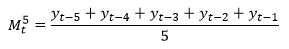
Moving Average

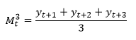
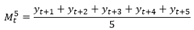
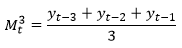
The moving average method is based on representing a series as a sum of sufficiently smooth trend and a random component.

The method is based on the local trend approximation using a polynomial of medium degree. To make trend assessment for the point t a polynomial of specified order p is selected for the series values within the time range [wt + w] using the least squares estimation method. Actually, this procedure is similar to calculating weighted sum of the series values at the range [ww] with the weights that depend on width of the interval 2 + 1 and order of the polynomial p. For a polynomial with the order p = 1 all weights are equal. This is one of the reasons why this method is named the moving averages method.

Moving averages need to be estimated when it is not clear, which function must be selected for a trend. The value of the moving average at t time is the arithmetic mean of the sequence of time series values on the time interval, the center of which is t point.

Define via Mtp the value of the moving average at t time determined by p points. For example:

And so on.

This makes obvious that the number of points p must be odd, otherwise the arithmetic mean must be attributed to a fractional point in time. However, in actual practice the number p is more conveniently selected as even. Then the arithmetic mean is calculated using some weights. For example, if we assume that p = 4, Mt4 can be calculated as follows:

The calculation of the moving average by four points amounted to the calculation by five points with the set of weights (1, 2, 2, 2, 1). The method of calculating moving average by the even number of points is named mean correction.

See also:

Modeling Container: The Moving Average Model | Time Series Analysis: Moving Average | IModelling.Movavg | ISmSlideSmoothing